Statistical Power
Plus alpha, beta, and the central limit theorem.
Statistical Power is your ability to detect an effect if there is one in a population. Say you’re testing whether the Firebolt is faster than the Nimbus 2001—which it obviously is, but let’s do this statistically. Statistical Power would be the probability of you rejecting the null (H0: there is no difference in speed) when there really is a difference in broom speed.
Hypothesis Tests
To understand power you need to understand hypothesis tests. When we use basic, inferential tests like the t–test or F–test, we ask wether the difference we observe is extreme enough to say that we are pretty sure it didn’t come from a population with no difference. We decide whether it’s sufficiently rare by comparing a) the probability that we would get this sample data if we were drawing randomly from a population where there is no difference to b) some threshold that we choose— called alpha (usually 0.05, aka 5%).
I’ve found an average difference of 12 MPH between the Firebolt and Nimbus (suck it, Malfoy); if there was no difference between the Firebolt and Nimbus in the population, how likely are we to get samples where the difference is 12 or larger? This is our p–value. Then we compare our p–value to our alpha. If our p–value is smaller than alpha, we reject the null hypothesis.
Type I Error (alpha)
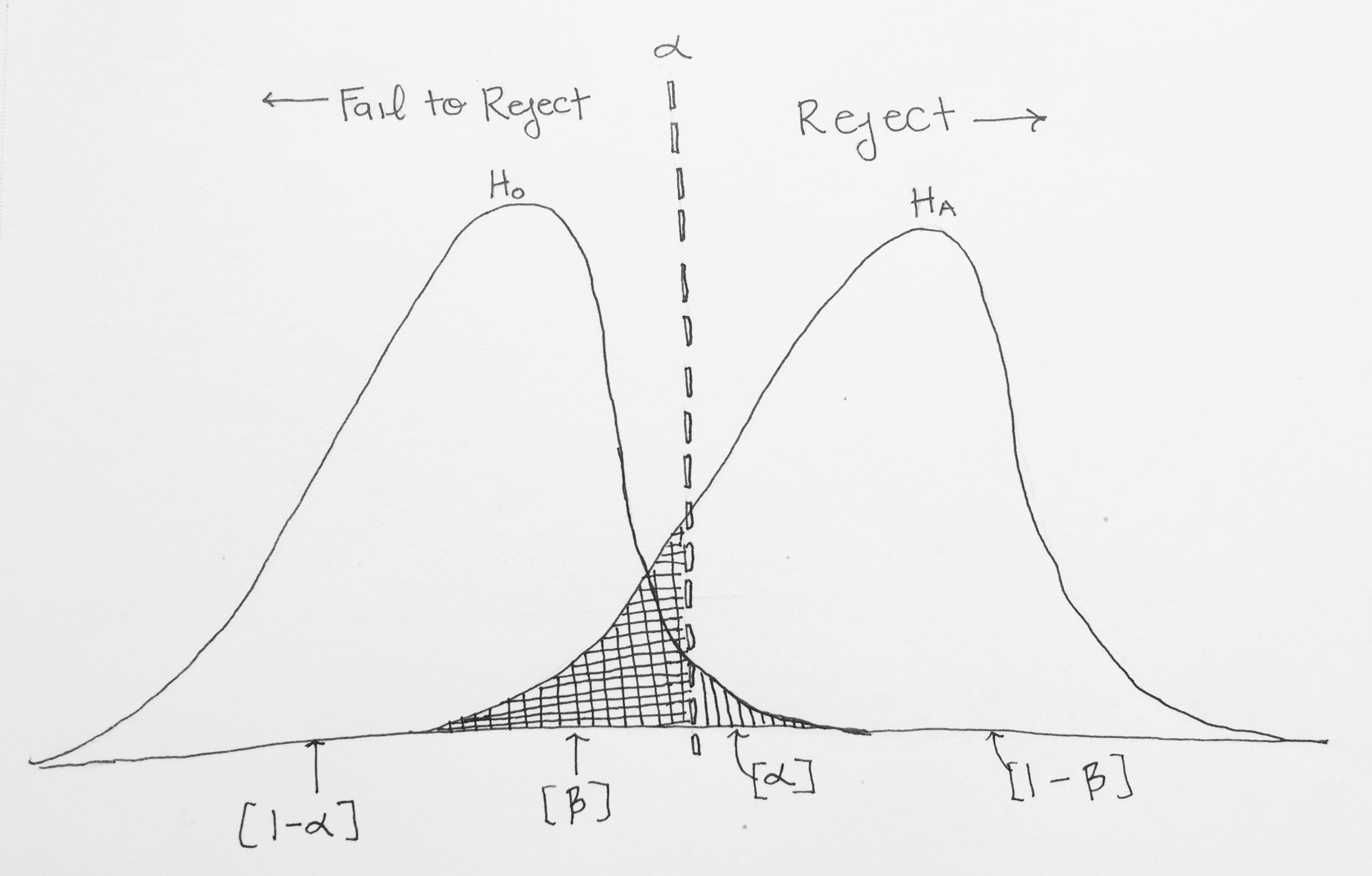
In the picture below, the vertical line represents our alpha level. It is placed so that 5% of the area in the null (H0) distribution is to the right of the vertical line. When we choose our alpha we know that if the null were true and there were no difference between the Firebolt and the Nimbus, 5% of the time we will get sample data that would have a big enough difference to lead us to reject the null even though the null is true. This is called a Type I error—the probability of rejecting the null even though it’s true. Our rate of Type I error is under our control, it’s always going to be the alpha we choose!
Type II error (Beta)
Also in this picture you see the alternative hypothesis distribution, Ha. In our example this would be the distribution of differences between the Firebolt and Nimbus if there were a certain difference between their speeds. It overlaps with the null distribution and more importantly, with the vertical line. Regardless of distributions, any difference in speed that is to the left of the vertical line will cause us to fail to reject the null, and anything to the right of the vertical line will cause us to reject the null. So, sometimes, we may fail to reject the null even though we should reject it (because Ha is true). This happens in the gridded region in the above picture (labeled Β). Β represents our Type II error—the probability of failing to reject the null even though it is false in the population.
Making the right Decision
Type I and II errors are when we make a decision that is not consistent with the population, but we can also make the correct choice too! We can either correctly keep the Null Hypothesis—if it’s true—or we can correctly Reject the Null Hypothesis—if it’s false. The proportion of the Null Distribution to the left of the line represents times when the Null is true and we correctly retain the Null. The probability of this will happen when the Null is really true is 1–alpha.
We can also correctly reject the null when it actually is false in the population. The Alternative Distribution represents the times when the Null Hypothesis is False, so anything in that distribution to the right of the line represents times when we correctly reject the Null. This…drumroll…is our Statistical Power: the ability to correctly detect an effect if there truly is one, and it’s probability is 1–Beta.
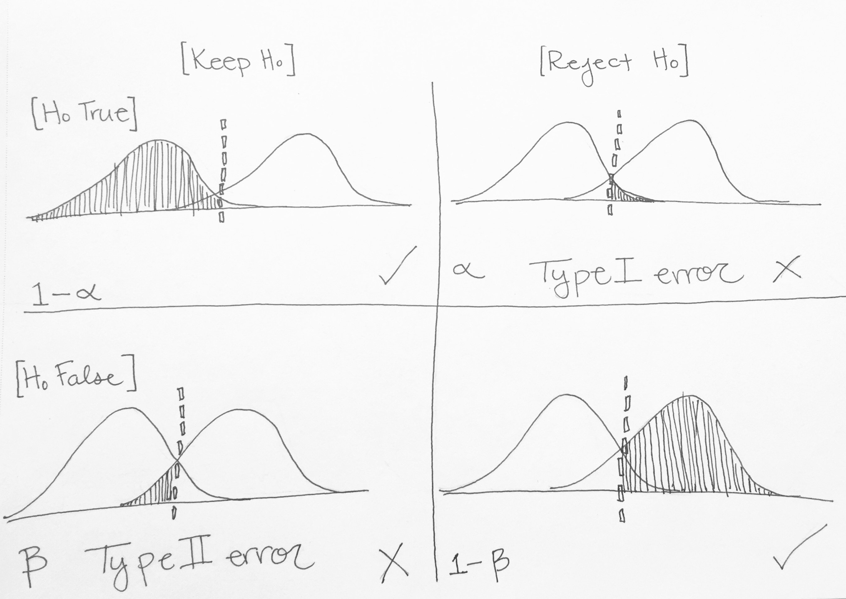
Power is pretty important, if you’re going to take the time to run a bunch of participants, fly a bunch of brooms, or grow a bunch of dishes of cells, you want to make sure that if there really is a difference then you’ll be able to detect it statistically. Visually you can see that the more the distributions overlap, the less power there will be since more of the alternative distribution will be to the left of the alpha cut off.
A few things can effect the overlap of the distributions—and therefore the power. Let’s go through them:
Effect Size: effect size will effect the spacing between the two distributions. If our brooms have a 12 MPH difference it will be easier to detect than a 4 MPH difference but harder to detect than a 34 MPH difference. We can’t control effect size, so I’ll give it 1 out of 5 stars for our ability to use this to change power. ★☆☆☆☆1

Alpha: alpha is the level of comparison for your p–value. If we had alpha = 0.10 then we would be shifting the line to the left which means that more of the Alternative Distribution would be to the right of the line, increasing power. However we would also be increasing our chances of making a Type I error. Fields usually have their own standards for alpha (0.05 is a popular one), so the only real way to change alpha is to switch from a 2–tailed test to a 1–tailed test. ★★☆☆☆
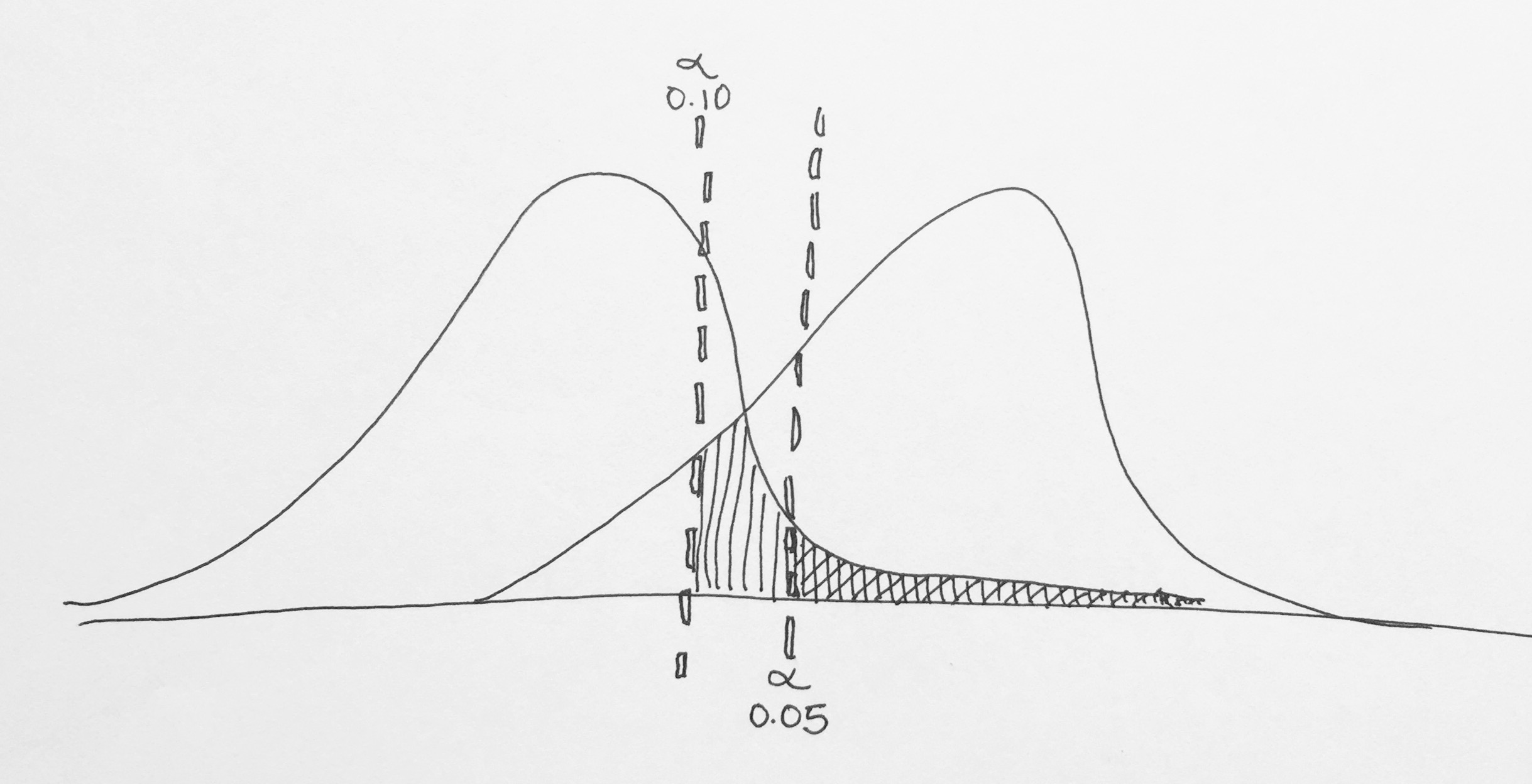
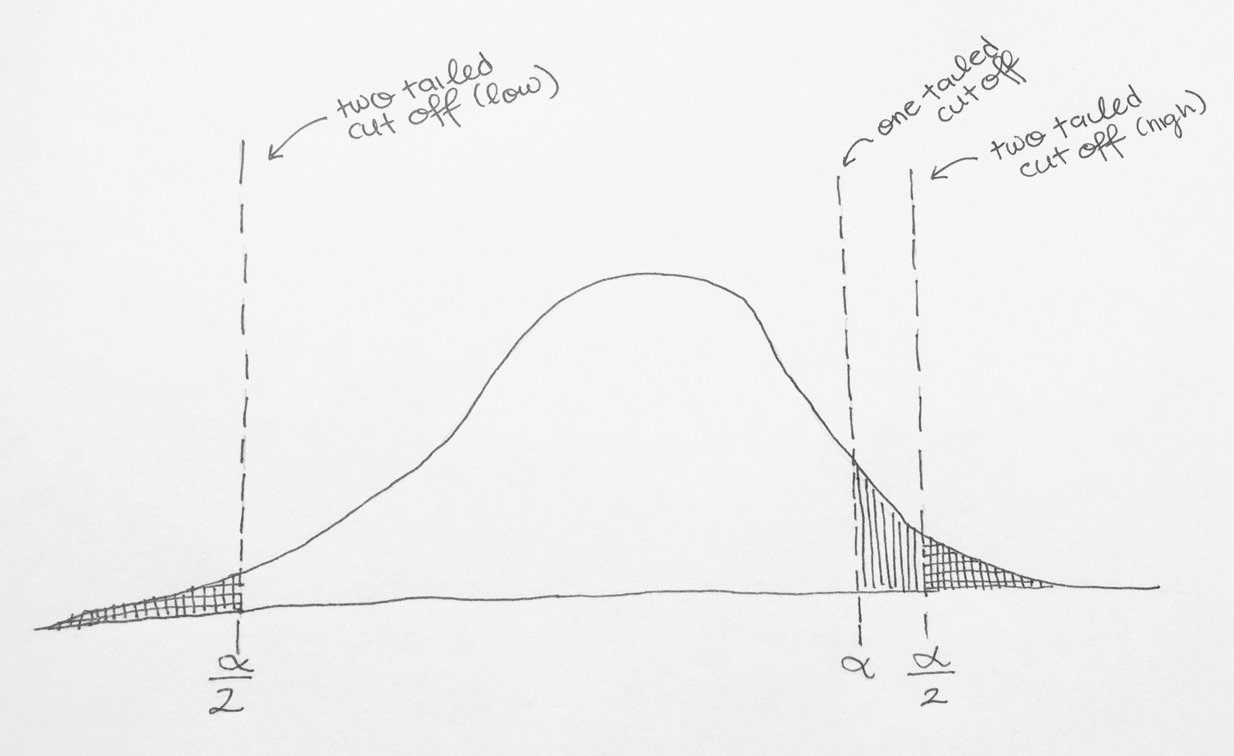
When we do a two-tailed test, we actually split our alpha into 2, one part for the lower tail and one for the upper tail. If your alpha is 0.05, then the top 2.5% of your distribution and the bottom 2.5% of your distribution will be in the “reject the Null” zone. Not splitting it would mean that all 5% could be on one tail—meaning that less extreme values would still be in the rejection region. Anything in the lined but not gridded area below are examples of samples where you would not reject the null with a 2-tailed test, but would with a 1-tailed test. Sometimes this is justified, but people can be skeptical when you use a 1-tailed test.
Sample Size: Ah, sample size. A researcher’s best friend. Increasing your sample size is completely in your control and will squeeze your Null and Alternative Distributions and make them skinnier (think Kardashian waist training). The skinnier they are, the less they will tend to overlap. This is because when you take the mean of larger samples, it’s harder to get extreme values and easier to get average ones; #throwback to the Central Limit Theorem. ★★★★☆
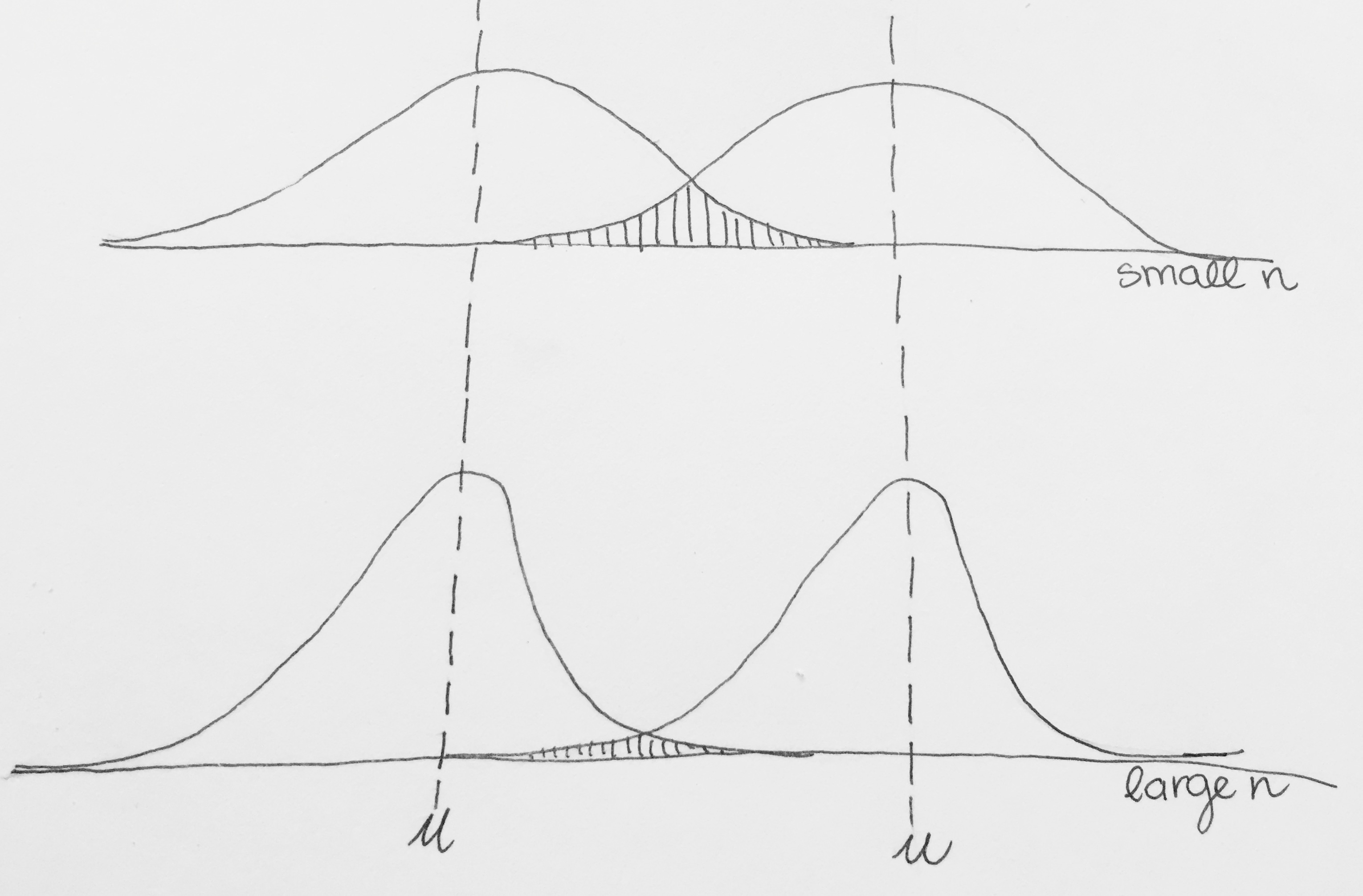
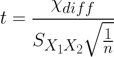
The math-y reason is that the error term in a distribution of sample means is the standard error or (pooled standard deviation for differences) which both have n in the denominator of their denominator—yikes that’s a mouthful! Basically the larger n is, the smaller the standard error/pooled standard deviation will be (which squeezes the distributions, remember Central Limit Theorem). The smaller those error terms are, the larger the t value will be, even though the difference between your two groups is the same!
So there you have it, statistical power in a nutshell. Go forth and analyze.
1 note: These stars are completely arbitrary and made up by the author for fun.
If you have any suggestions for topics you’d like to see in the Data Science Dictionary, feel free to reach out! The preferred form of request is “What the heck is ______?”
